Overview

The Solver configuration workspace defines the temporal structure of a simulation and controls how the system state is propagated over time within SatModeler.

Within this workspace, users configure the simulation start date, total simulation duration, and the numerical integration time step. These parameters establish the global time reference used by the simulation engine and determine how all physical models, subsystems, and onboard algorithms evolve in time.

The solver configuration directly affects:

• Time reference and timestamping of the simulation
• Numerical propagation of spacecraft dynamics
• Python script callbacks and exported logs
• Determinism and reproducibility of simulation results

This configuration is typically defined once per mission and applies globally to all spacecraft and subsystems involved in the simulation.

Main Features

Simulation Time Configuration

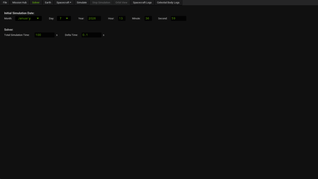
The simulation time configuration is defined by two complementary parameters: the initial simulation date and the total simulation duration.

• Initial Simulation Date (UTC)
  Establishes the UTC reference epoch from which the simulation starts.
  The seconds field supports sub-second resolution up to microseconds, enabling precise temporal alignment when simulating high-frequency dynamics, sensors, or event-driven onboard logic.
• Total Simulation Time
  Defines the overall duration of the simulation, expressed in seconds. The solver advances the simulation state from the initial epoch until the specified total time is reached.

Together, these parameters define the absolute timing and the temporal extent of the simulation and directly influence the length and time span of all generated logs and exported data.

Discrete-Time Integration Step

The integration time step defines the fixed time increment used by the solver to advance the simulation state.

SatModeler employs a discrete-time numerical integration approach, meaning that the simulation progresses in uniform, fixed-duration steps. This design choice is intentional and provides a deterministic temporal structure across the entire simulation.

Key characteristics of this approach include:

• Deterministic timestamps in all simulation logs and exported data
• Predictable execution of Python-bound algorithms, always triggered at known and repeatable time instants
• Reproducible simulations, essential for validation, debugging, and comparative analysis

At each integration step, the spacecraft state is propagated using a multi-stage numerical integration scheme. As part of this process, user-created Python scripts may be evaluated multiple times internally within a single time step to ensure numerical accuracy.

This solver architecture is particularly well suited for simulations involving:

• Sensor modeling and signal processing
• State estimation algorithms
• Guidance, navigation, and control systems
• Power, thermal, and communication subsystems
• Onboard software logic executed via Python bindings

Smaller integration time steps improve numerical accuracy and temporal resolution but increase computational cost. Larger steps reduce execution time at the expense of reduced fidelity.

Additional integration schemes may be introduced in future versions of SatModeler to support different simulation requirements.

Choosing a Stable Integration Time Step (Δt)

A practical way to select Δt is to identify the fastest dynamics in your simulation (i.e. the highest relevant frequency) and choose a time step small enough to resolve it with sufficient margin.

In practice, stability and accuracy depend on how well the integration time step captures these fast dynamics. If Δt is too large, numerical errors may accumulate, leading to unstable behavior or loss of fidelity in the simulation results.

Useful Rules of Thumb

The following guidelines provide practical estimates for selecting a stable and accurate integration time step based on common spacecraft simulation scenarios.

Fastest dynamics driver	Parameter to estimate	Recommended time step (Δt)	Rationale
Orbit propagation (translation) (e.g. position/velocity only, long-duration runs)	Orbital period T (s) or mean motion n = 2π / T (rad/s)	Δt ≤ T / 1000 (use T / 2000 for higher fidelity)	Provides sufficient resolution over an orbit for smooth position and velocity propagation. Note that SatModeler still integrates attitude, so the time step may need to be smaller if the spacecraft angular rate is high.
Attitude kinematics (rotation) (e.g. fast slews, detumbling, precise pointing)	Maximum spacecraft angular rate ωmax (rad/s)	Δt ≤ 0.1 / ωmax (keep per-step rotation small, e.g. < 0.1 rad)	Limits how much the spacecraft can rotate in a single step, keeping attitude propagation smooth and avoiding large numerical errors.
Oscillatory dynamics (e.g. flexible appendages, structural modes)	Highest natural frequency of the system fn (Hz), with ωn = 2πfn (rad/s)	Δt ≲ 2.8 / ωn	Ensures that oscillatory motion is properly resolved and does not grow artificially due to numerical instability.
Accuracy-driven signals (e.g. sensor/actuator models implemented in Python)	Highest signal or model update frequency fmax (Hz)	Δt ≤ 1 / (20 · fmax) (1 / (50 · fmax) for high fidelity)	Provides enough time resolution to capture fast variations without excessive phase lag or loss of signal detail.
Python logic / control loops (e.g. onboard estimation and control algorithms)	Controller or algorithm update rate fc (Hz)	Δt ≤ 1 / (10 · fc)	Keeps Python callbacks deterministic and well synchronized with the simulated dynamics and control updates.

If multiple criteria apply, always select the smallest Δt. The simulation time step should be driven by the fastest dynamics present in the system.

How to Use

1. Set the initial simulation date and time (UTC), including sub-second precision if required. This defines the global time reference for the simulation.
2. Define the total simulation time, in seconds, according to the duration of the scenario to be analyzed.
3. Select an appropriate integration time step. For simulations involving sensors, estimation, control, or onboard algorithms executed via Python, a fixed and sufficiently small time step is recommended to ensure accurate timing, deterministic behavior, and proper synchronization across subsystems.

Once configured, the solver settings are applied automatically by SatModeler and remain active throughout the simulation without further user intervention.